Technical Interview Cheat Sheet

I’ve been working on a fork of TSiege’s gist on studying for technical interviews on and off for the last six months or so. I modified it to fit the format from Cracking the Coding Interview a bit better. Hope you get something out of this – I’ll probably repost it on the UO Dev Club blog soon.

Programming interviews are both about displaying your command of programming fundamentals, as well as taking those fundamentals and applying them to a problem you’ve never seen before. The better your fundamentals, the better it will go. The fundamentals break down into two or three major categories: data structures, algorithms, and the concepts underlying why those data structures and algorithms are optimal.

This list is meant to be both a quick guide and reference for further research into these topics. There’s no way we can cover everything in depth with just a cheat sheet. If you’re unfamiliar with any of the terms below, take it upon yourself to learn the content better. If anything under here is unfamiliar, you’re very vulnerable to having the holes in your knowledge seen in a programming interview. If you have command of everything in this section, you have the foundation required to solve most, if not any, problem thrown at you.

First, I must warn you: in order to even make it to this point, you will need to pass a phone screen, first interview, or some other “soft skills” interview. The skills needed to succeed are not covered here, but I’ll give a quick summary on this:

Have strong intellectual control over the projects you’ve worked with. This means you need to know all the typical questions – “What was the hard part?” “What did you do?” “Tell me about the biggest challenge you had.” Be able to answer any question about two or three major projects you’ve worked on. For internships at many companies (meaning: not a destination company), this will be your ENTIRE interview. If you can thoroughly explain your projects and have solid answers for soft questions like these, your chances of making it to the next round are far increased.

With no further ado, the Technical Interview Cheat Sheet!

Data Structures and Types

Linked List

Definition:

Stores data with nodes that point to other nodes.
- Nodes, at their most basic, have one datum and one reference (the next node, generally next).
- A linked list chains nodes together by pointing one node’s reference towards another node.

What you need to know:

Designed to optimize insertion and deletion, slow at indexing and searching.
Doubly linked lists have nodes that reference the previous node in addition to the next node.
A circularly linked list is simple linked list whose tail, the last node, references the head, the first node.
Stacks are commonly implemented with linked lists, but can also be made from arrays.
- Stacks are last in, first out (LIFO) data structures.
- Made with a linked list by having the head be the only place for insertion and removal.
- Array implementation pushes and pops to the end of the array, with another variable tracking the final index position.
Queues, too, can be implemented with a linked list or an array.
- Queues are a first in, first out (FIFO) data structure.
- Made with a doubly linked list that only removes from head and adds to tail.
- Array implementation pushes to end of array and pops from front of array. Two variables needed, to track front and back of queue. If you’re really swanky, you can use the array circularly.

Operations w/ Big O efficiency

Linked lists are a chain of nodes; operations are performed on the nodes.

.next and .prev: O(1) operations.
Search: O(n), performed by .next and .prev operations.
Indexing: O(n), performed by .next and .prev operations.
Insertion: O(n) if anywhere but beginning, performed by .next and .prev operations.
- Insertion at beginning is O(1).
Deletion: O(n) if anywhere but beginning, performed by .next and .prev operations.
- Deletion at beginning is O(1).

Binary Tree

Definition:

Is a data structure composed of connected nodes, where each node has at most two children (left and right).
- “N-ary” trees, including prefix trees (tries), have more than two children. Those are covered later.

What you need to know:

Designed to optimize searching and sorting.
A degenerate tree is an unbalanced tree, which if entirely one-sided is a essentially a linked list.
They are comparably simple to implement than other data structures.
Used to make binary search trees and binary heaps.
Multiple implementation options:
- Node-based: literal left / right / parent nodes, implemented as independent data structures to make up a binary tree.
- Array-based: uses indices and basic arithmetic (node_index*2 is left, *2+1 is right) to keep track of parents and children.

Operations w/ Big O efficiency:

Binary Trees are collections of left and right child nodes, beginning at a parent node.

.left, .right, .parent: O(1) operations to reach a known connected node.
Indexing: Binary Search Tree: O(log n) Binary Tree: O(n)
Search: Binary Search Tree: O(log n) Binary Tree: O(n)
Insertion: Binary Search Tree: O(log n) Binary Tree: O(n)

Binary Heap

Definition

Specific implementation of a Binary Tree, organized by some priority; generally a “min-heap” or “max-heap”.
Implementations must maintain the heap property and shape property.
- Heap Property: All nodes are either greater than or equal to (max-heap) or less than or equal to (min-heap) each of its children, according to a comparison predicate defined for the heap.
- Shape Property: A binary heap is a complete binary tree, and if the last level of the tree is not complete, the nodes of that level are filled from left to right.

What you need to know:

Priority queues are often implemented using a heap of some form.
Heapsort takes advantage of in-place operations in an array and heap property to sort in O(n log n) time.

Binary Search Tree

Definition

Specific implementation of a Binary Tree.

What you need to know:

A binary tree that uses comparable keys to assign which direction a child is.
Left child has a key smaller than it’s parent node.
Right child has a key greater than it’s parent node.
There can be no duplicate node.
Because of the above it is more likely to be used as a data structure than a binary tree.

Array

Definition:

Stores data elements based on an sequential, most commonly 0 based, index.
Based on tuples from set theory.
They are one of the oldest, most commonly used data structures.

What you need to know:

Optimal for indexing; bad at searching, inserting, and deleting (except at the end).
Linear arrays, or one dimensional arrays, are the most basic.
- Static in size, meaning that they are declared with a fixed size.
Dynamic arrays (Vectors / ArrayLists) are like one dimensional arrays, but have reserved space for additional elements.
- If a dynamic array is full, it copies it’s contents to a larger array.
Two dimensional arrays have x and y indices like a grid or nested arrays.
Arrays can be used to implement both stacks and queues, as covered above in the Linked List section.

Big O efficiency:

Indexing: Linear array: O(1), Dynamic array: O(1)
Linear Search: Linear array: O(n), Dynamic array: O(n)
Sorted Search: Linear array: O(log n), Dynamic array: O(log n)
Insertion: Linear array: n/a Dynamic array: O(n)

Hash Table or Hash Map

Definition:

Stores data with key value pairs.
Hash functions accept a key and return an output unique only to that specific key.
- This is known as hashing, which is the concept that an input and an output have a one-to-one correspondence to map information.
- Hash functions return a unique address in memory for that data.

What you need to know:

Designed to optimize searching, insertion, and deletion.
Hash collisions are when a hash function returns the same output for two distinct outputs.
- All hash functions have this problem.
- This is often accommodated for by having the hash tables be very large.
Hashes are important for associative arrays and database indexing.

Big O efficiency:

Indexing: Hash Tables: O(1)
Search: Hash Tables: O(1)
Insertion: Hash Tables: O(1)

Prefix Trees (Tries)

Definition

A specific kind of “n-ary” tree, storing words (and prefixes to those words).
Each node contains a letter and references to other letter nodes if that node is part of a prefix to another word.
If a letter node is also the last one in a word, it should contain data saying so.

What you need to know:

These are NOT something you’re likely to have met in school, but can be a very practical relative of the “n-ary” tree.
This is the best way to implement a dictionary of words, unless you can throw unrealistic amounts of money at the problem.
At a minimum, it supports “insert word,” “search for word,” and “starts with” operations.
Besides implementing a dictionary of words, or something with similar prefixes, this structure may not give you much mileage.

Big-O Efficiency

Search: Prefix Trees: O(n)
Insertion: Prefix Trees: O(n)

Graphs

Definition:

Specifies relationships among a collection of items.
Consists of a set of objects called nodes.
Related nodes are connected by edges.
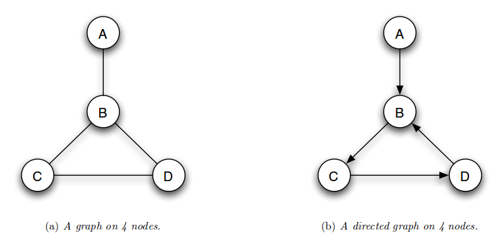
Graphs can be either directed or undirected.
- A directed graph has directed edges, signifying a one-way relationship between nodes. There can be a directed edge one way and another directed edge back toward the node of origin, but they are distinct and different edges.
- An undirected graph has undirected edges, signifying a two-way relationship between nodes. Traversal one way is the same as traversal on the way back; it is the same edge. These are far more common than directed graphs, and as such is the default when we refer to a generic graph.

*Image Credit: David Easley and Jon Kleinberg*

What you need to know:

Graphs are ubiquitous in both theoretical and applied computer science.
- As such, many many algorithms are already standard for handling graphs: Djikstra’s, breadth-first or depth-first search, Floyd-Warshall, etc.
Trees can be thought of as graphs; the connnections between nodes are edges that can normally be traversed both ways equally through the parent-child relationship. Most algorithms that apply to one can be applied to the other as well.

Big O efficiency:

Graphs are an abstract data type that is generally represented by something between a tree and linked list. Whatever you choose in that regard will maintain its Big O properties, plus however you choose to represent the Node and Edge.

Example:

TODO: This would probably be a good idea to represent since there is so much variability in implementation.

Add to this section…

Other N-ary trees, oddball questions

Algorithms: Search

Breadth First Search

Definition:

An algorithm that searches a tree (or graph) by searching levels of the tree first, starting at the root.
- It finds every node on the same level, most often moving left to right.
- While doing this it tracks the children nodes of the nodes on the current level.
- When finished examining a level it moves to the left most node on the next level.
- The bottom-right most node is evaluated last (the node that is deepest and is farthest right of it’s level).

What you need to know:

Optimal for searching a tree that is wider than it is deep.
Uses a queue to store information about the tree while it traverses a tree.
- Because it uses a queue it is more memory intensive than depth first search.
- The queue uses more memory because it needs to stores pointers

Big O efficiency:

Search: Breadth First Search: O(|E| + |V|)
E is number of edges
V is number of vertices

Depth First Search

Definition:

An algorithm that searches a tree (or graph) by searching depth of the tree first, starting at the root.
- It traverses left down a tree until it cannot go further.
- Once it reaches the end of a branch it traverses back up trying the right child of nodes on that branch, and if possible left from the right children.
- When finished examining a branch it moves to the node right of the root then tries to go left on all it’s children until it reaches the bottom.
- The right most node is evaluated last (the node that is right of all it’s ancestors).

What you need to know:

Optimal for searching a tree that is deeper than it is wide.
Uses a stack to push nodes onto.
- Because a stack is LIFO it does not need to keep track of the nodes pointers and is therefore less memory intensive than breadth first search.
- Once it cannot go further left it begins evaluating the stack.

Big O efficiency:

Search: Depth First Search: O(|E| + |V|)
E is number of edges
V is number of vertices

Breadth First Search vs. Depth First Search

The simple answer to this question is that it depends on the size and shape of the tree.
- For wide, shallow trees use Breadth First Search
- For deep, narrow trees use Depth First Search

Nuances:

Because BFS uses queues to store information about the nodes and its children, it could use more memory than is available on your computer. (But you probably won’t have to worry about this.)
If using a DFS on a tree that is very deep you might go unnecessarily deep in the search. See this xkcd for more information.
Breadth First Search tends to be a looping algorithm.
Depth First Search tends to be a recursive algorithm.

Binary Search

Definition

Executed on a sorted array, this is an O(log n) search algorithm for arrays that mimics the structure of a balanced BST.
In a while loop, start by checking the middle index (max + low / 2) for your value.
- If array[mid] == your value, woo! You’re done.
- If array[mid] > your value, it can’t be any higher than that on the array. Upper bound of array is the previous minimum minus one.
- If array[mid] < your value, it can’t be any lower than that on the array. Lower bound of array is the previous minimum plus one.

What you need to know:

Be careful on how you calculate min, and watch the +1 / -1 on upper and lower bounds. Those off-by-one errors are nasty.

Big O Efficiency:

Binary Search is a O(log n) operation.

Algorithms: Sorting

Merge Sort

Definition:

A comparison based sorting algorithm
- Divides entire dataset into groups of at most two.
- Compares each number one at a time, moving the smallest number to left of the pair.
- Once all pairs sorted it then compares left most elements of the two leftmost pairs creating a sorted group of four with the smallest numbers on the left and the largest ones on the right.
- This process is repeated until there is only one set.

What you need to know:

This is one of the most basic sorting algorithms.
Know that it divides all the data into as small possible sets then compares them.
Natural merge sort, a variant, exploits existing runs of sorted data to approach O(n) best case.
- This is a key component of Timsort, the sort of choice in the Python standard library.

Big O efficiency:

Best Case Sort: Merge Sort: O(n log n), unless natural variant
Average Case Sort: Merge Sort: O(n log n)
Worst Case Sort: Merge Sort: O(n log n)

Quicksort

Definition:

A comparison based sorting algorithm
- Divides entire dataset in half by selecting the average element and putting all smaller elements to the left of the average.
- It repeats this process on the left side until it is comparing only two elements at which point the left side is sorted.
- When the left side is finished sorting it performs the same operation on the right side.
Computer architecture favors the quicksort process.

What you need to know:

While it has the same Big O as (or worse in some cases) many other sorting algorithms it is often faster in practice than many other sorting algorithms, such as merge sort.
Know that it halves the data set by the average continuously until all the information is sorted.

Big O efficiency:

Best Case Sort: Merge Sort: O(n)
Average Case Sort: Merge Sort: O(n log n)
Worst Case Sort: Merge Sort: O(n^2)

Bubble Sort

Definition:

A comparison based sorting algorithm
- It iterates left to right comparing every couplet, moving the smaller element to the left.
- It repeats this process until it no longer moves and element to the left.

What you need to know:

While it is very simple to implement, it is the least efficient of these three sorting methods.
Know that it moves one space to the right comparing two elements at a time and moving the smaller on to left.

Big O efficiency:

Best Case Sort: Merge Sort: O(n)
Average Case Sort: Merge Sort: O(n^2)
Worst Case Sort: Merge Sort: O(n^2)

Merge Sort Vs. Quicksort

Quicksort is likely faster in practice.
Merge Sort divides the set into the smallest possible groups immediately then reconstructs the incrementally as it sorts the groupings.
Quicksort continually divides the set by the average, until the set is recursively sorted.

Concepts: Algorithms

Recursive Algorithms

Definition:

An algorithm that calls itself in its definition.
- Recursive case a conditional statement that is used to trigger the recursion.
- Base case a conditional statement that is used to break the recursion.

What you need to know:

Stack level too deep and stack overflow.
- If you’ve seen either of these from a recursive algorithm, you messed up.
- It means that your base case was never triggered because it was faulty or the problem was so massive you ran out of RAM before reaching it.
- Knowing whether or not you will reach a base case is integral to correctly using recursion.
- Often used in Depth First Search

Iterative Algorithms

Definition:

An algorithm that is called repeatedly but for a finite number of times, each time being a single iteration.
- Often used to move incrementally through a data set.

What you need to know:

Generally you will see iteration as loops, for, while, and until statements.
Think of iteration as moving one at a time through a set.
Often used to move through an array.

Recursion Vs. Iteration

The differences between recursion and iteration can be confusing to distinguish since both can be used to implement the other. But know that,
- Recursion is, usually, more expressive and easier to implement.
- Iteration uses less memory.
Functional languages tend to use recursion. (i.e. Haskell)
Imperative languages tend to use iteration. (i.e. Ruby)
Check out this Stack Overflow post for more info.

Pseudo Code of Moving Through an Array (this is why iteration is used for this)

Recursion                         | Iteration
----------------------------------|----------------------------------
recursive method (array, n)       | iterative method (array)
  if array[n] is not nil          |   for n from 0 to size of array
    print array[n]                |     print(array[n])
    recursive method(array, n+1)  |
  else                            |
    exit loop                     |

Greedy Algorithm

Definition:

An algorithm that, while executing, selects only the information that meets a certain criteria.
The general five components, taken from Wikipedia:
- A candidate set, from which a solution is created.
- A selection function, which chooses the best candidate to be added to the solution.
- A feasibility function, that is used to determine if a candidate can be used to contribute to a solution.
- An objective function, which assigns a value to a solution, or a partial solution.
- A solution function, which will indicate when we have discovered a complete solution.

What you need to know:

Used to find the optimal solution for a given problem.
Generally used on sets of data where only a small proportion of the information evaluated meets the desired result.
Often a greedy algorithm can help reduce the Big O of an algorithm.

Pseudo Code of a Greedy Algorithm to Find Largest Difference of any Two Numbers in an Array.

greedy algorithm (array)
  var largest difference = 0
  var new difference = find next difference (array[n], array[n+1])
  largest difference = new difference if new difference is > largest difference
  repeat above two steps until all differences have been found
  return largest difference

This algorithm never needed to compare all the differences to one another, saving it an entire iteration.

To be added…

Dynamic Programming
Big O: Time and Space
Memory Management: Stack vs Heap
Bit Manipulation